Diving into dependen-“sea”

How CRAN packages are interconnected

H. Sherry Zhang

2022-10-18

When writing a package, we may want to use functions in other packages. This creates a dependency for our package and a reverse dependency on the package we borrow functions from. As one of the recipients of the isoband email¹, I’m curious to know how interconnected CRAN packages are. Luckily, it is not too hard to get data on this, and so the journey begins…

Preparing dependency data

The utils package provides the function available.packages() to extract CRAN package information. The data includes information on the package name, version, dependency, and license:

Code

(raw <- utils::available.packages() %>% as_tibble())

# A tibble: 18,692 × 17
   Package     Version Priority Depends  Imports Linki…¹ Sugge…² Enhan…³ License
   <chr>       <chr>   <chr>    <chr>    <chr>   <chr>   <chr>   <chr>   <chr>  
 1 A3          1.0.0   <NA>     R (>= 2… <NA>    <NA>    random… <NA>    GPL (>…
 2 AATtools    0.0.2   <NA>     R (>= 3… magrit… <NA>    <NA>    <NA>    GPL-3  
 3 ABACUS      1.0.0   <NA>     R (>= 3… ggplot… <NA>    rmarkd… <NA>    GPL-3  
 4 abbreviate  0.1     <NA>     <NA>     <NA>    <NA>    testth… <NA>    GPL-3  
 5 abbyyR      0.5.5   <NA>     R (>= 3… httr, … <NA>    testth… <NA>    MIT + …
 6 abc         2.2.1   <NA>     R (>= 2… <NA>    <NA>    <NA>    <NA>    GPL (>…
 7 abc.data    1.0     <NA>     R (>= 2… <NA>    <NA>    <NA>    <NA>    GPL (>…
 8 ABC.RAP     0.9.0   <NA>     R (>= 3… graphi… <NA>    knitr,… <NA>    GPL-3  
 9 abcADM      1.0     <NA>     <NA>     Rcpp (… Rcpp, … <NA>    <NA>    GPL-3  
10 ABCanalysis 1.2.1   <NA>     R (>= 2… plotrix <NA>    <NA>    <NA>    GPL-3  
# … with 18,682 more rows, 8 more variables: License_is_FOSS <chr>,
#   License_restricts_use <chr>, OS_type <chr>, Archs <chr>, MD5sum <chr>,
#   NeedsCompilation <chr>, File <chr>, Repository <chr>, and abbreviated
#   variable names ¹​LinkingTo, ²​Suggests, ³​Enhances

From this, we can extract a table to map out the direct dependency every CRAN package has. In this post we will focus on the two strong dependencies: Depends and Imports:

Code

all_pkgs <- raw %>% 
  tidyr::separate_rows(Imports, sep = ",") %>% 
  tidyr::separate_rows(Depends, sep = ",") %>% 
  mutate(
    across(c(Depends, Imports), ~gsub("\\(.*\\)", "\\1", .x)),
    across(c(Depends, Imports), str_trim)
    )
  # filter(!Depends %in% c("R", ""), Imports != "", !is.na(Depends))

(dep_lookup_tbl <- all_pkgs %>% 
  dplyr::select(Package, Depends, Imports) %>% 
  rename(downstream = Package) %>% 
  pivot_longer(Depends:Imports, names_to = "type", values_to = "upstream") %>% 
  distinct() %>% 
  filter(!upstream %in% c("R", "")) %>% 
  filter(!is.na(upstream)) %>% 
  arrange(downstream))

# A tibble: 96,765 × 3
   downstream type    upstream  
   <chr>      <chr>   <chr>     
 1 A3         Depends xtable    
 2 A3         Depends pbapply   
 3 AATtools   Imports magrittr  
 4 AATtools   Imports dplyr     
 5 AATtools   Imports doParallel
 6 AATtools   Imports foreach   
 7 ABACUS     Imports ggplot2   
 8 ABACUS     Imports shiny     
 9 ABC.RAP    Imports graphics  
10 ABC.RAP    Imports stats     
# … with 96,755 more rows

Dependency is a transitive relation. This means a package also (indirectly) depends on all the dependencies of the package of it imports and so on. Changes from an package will propagate downwards through its dependency chain. With the direct dependency table above, we can iteratively construct the extended dependency tree:

Code

find_all_deps <- function(upstream, data){
  print(upstream)
  dt <- tibble()
  dt2 <- data
  i <- 1
  while(nrow(dt2) > nrow(dt)){
    print(i)
    dt <- dt2
    n <- paste0("upstream", i) 
    dt2 <- dt %>% 
      rename(upstream = downstream) %>% 
      left_join(dep_lookup_tbl %>% select(-type), by = "upstream") %>% 
      rename(!!quo_name(n) := upstream)
    i <- i + 1
  }
  
  dep <- dt2 %>%
    pivot_longer(
      cols = c(contains("upstream"),  "downstream"),
      names_to = "dump", values_to = "downstream") %>%
    distinct(downstream) %>%
    filter(!is.na(downstream)) %>%
    mutate(downstream = sort(downstream))
  return(dep)
}

dep_all <- dep_lookup_tbl %>% 
  arrange(-desc(upstream)) %>% 
  nest(direct_deps = -upstream) %>% 
  mutate(all_deps = map2(upstream, direct_deps, find_all_deps))

(edges <- dep_all %>% 
    select(-direct_deps) %>% 
    unnest(all_deps) %>% 
    filter(!is.na(upstream), !is.na(downstream)))

# A tibble: 551,713 × 2
   upstream downstream
   <chr>    <chr>     
 1 a4Core   nlcv      
 2 abc      abctools  
 3 abc      EasyABC   
 4 abc      ecolottery
 5 abc      nlrx      
 6 abc      paleopop  
 7 abc      poems     
 8 abc.data abc       
 9 abc.data abctools  
10 abc.data EasyABC   
# … with 551,703 more rows

The plot below shows the number of dependencies and reverse dependencies a package has.

Code

nodes <- tibble(id = unique(c(edges$upstream, edges$downstream))) %>% 
  left_join(edges %>% count(upstream, name = "n_revdep"), by = c("id" = "upstream")) %>% 
  left_join(edges %>% count(downstream, name = "n_dep"), by = c("id" = "downstream")) %>% 
  filter(!is.na(id)) %>% 
  mutate(n_revdep = ifelse(is.na(n_revdep), 0, n_revdep),
         n_dep = ifelse(is.na(n_dep), 0, n_dep))

################################################################
# deriving color categories
recommended <- raw %>% filter(Priority == "recommended") %>% pull(Package)

base <- c("base", "compiler", "datasets", "grDevices", "graphics", "grid", "methods", "parallel", "splines", "stats", "stats4", "tcltk", "tools", "translations", "utils")

r_lib_gh <- gh("GET /orgs/{username}/repos", username = "r-lib", .limit = 200)
r_lib <- vapply(r_lib_gh, "[[", "", "name")

r_tidyverse_gh <- gh("GET /orgs/{username}/repos", username = "tidyverse", .limit = 40)
tidyverse <- vapply(r_tidyverse_gh, "[[", "", "name")

nodes <- nodes %>% 
  mutate(category = 
           case_when(id %in% tidyverse ~ "tidyverse", 
                     id %in% base ~ "base",
                     id %in% r_lib ~ "r-lib",
                     id %in% recommended ~ "recommended",
                     TRUE ~ "zzz"))
################################################################
# to deal with zero mark after sqrt tranform
# https://github.com/tidyverse/ggplot2/issues/980
mysqrt_trans <- function() {
    scales::trans_new("mysqrt", 
              transform = base::sqrt,
              inverse = function(x) ifelse(x<0, 0, x^2),
              domain = c(0, Inf))
}

p <- nodes %>% 
  mutate(tooltip = glue::glue("Pkg: {id}, dep: {n_dep}, revdep: {n_revdep}")) %>% 
  ggplot(aes(x = n_dep, y = n_revdep)) + 
  geom_point_interactive(aes(tooltip = tooltip)) +
  ggrepel::geom_text_repel(
    data = nodes %>% filter(n_revdep > 3100),
    aes(color= category, label = id), min.segment.length = 0) +
  scale_color_brewer(palette = "Set1") + 
  scale_y_continuous(breaks = c(0,  50, 200, 500, 1000, 2500, 5000, 7500, 10000, 15000), trans = "mysqrt") + 
  scale_x_continuous(breaks = c(0, 1, 5, 10, 20, 40, 80, 120, 160, 200), trans = "mysqrt") + 
  theme(panel.grid.minor = element_blank(),
        legend.position = "bottom") + 
  xlab("Number of dependencies") + 
  ylab("Number of reverse dependencies")

girafe(ggobj = p, width_svg = 16, height_svg = 12)

The x and y-axes show the number of dependencies and reverse dependencies of a package. Both coordinates are square root transformed to accommodate for the skewness in both measures. Packages with more than 3100 reverse dependencies are labelled. The label color denotes four groups: those in base R, those labelled as “recommended” by CRAN, and those listed in the tidyverse and r-lib organisations on GitHub. Expand the color group below to view the package membership:

color group

category	packages
base	base, compiler, datasets, graphics, grDevices, grid, methods, parallel, splines, stats, stats4, tcltk, tools, utils
tidyverse	blob, dbplyr, dplyr, dtplyr, forcats, ggplot2, glue, googledrive, googlesheets4, haven, hms, lubridate, magrittr, modelr, multidplyr, nycflights13, purrr, readr, readxl, reprex, rvest, stringr, tibble, tidyr, tidyverse, vroom
r-lib	archive, askpass, available, backports, bench, brio, cachem, callr, carrier, cli, clisymbols, clock, commonmark, conflicted, coro, covr, cpp11, crayon, credentials, debugme, desc, devtools, downlit, ellipsis, err, evaluate, fastmap, filelock, fs, gargle, generics, gert, gh, gitcreds, gmailr, gtable, here, httr, httr2, jose, keyring, later, lifecycle, lintr, liteq, lobstr, memoise, mockery, pak, pillar, pingr, pkgbuild, pkgcache, pkgconfig, pkgdepends, pkgdown, pkgload, prettycode, prettyunits, processx, progress, ps, R6, ragg, rappdirs, rcmdcheck, rematch2, remotes, rex, rlang, roxygen2, rprojroot, scales, sessioninfo, showimage, sodium, styler, svglite, systemfonts, testthat, textshaping, tidyselect, tzdb, urlchecker, usethis, vctrs, waldo, whoami, withr, xml2, xmlparsedata, xopen, ymlthis, zeallot, zip, roxygen2md, diffviewer, vdiffr, asciicast, cliapp, decor, meltr, sloop, tracer, io, conf, webfakes
recommended	boot, class, cluster, codetools, foreign, KernSmooth, lattice, MASS, Matrix, mgcv, nlme, nnet, rpart, spatial, survival

The plot is interactive so you can hover over points of your interest to read the package name and its numbers of (reverse) dependency.

It’s okay to be a couch Pareto

As you would have already noticed, the distribution of the number of reverse dependencies is highly skewed, even after the square root transformation. To better visualise how the lower number of reverse dependency is distributed, we can plot its cumulative distribution:

Code

prct_tbl <- purrr::map_dfr(
  unique(nodes$n_revdep) %>% sort(), 
  ~tibble(n = .x, prct = nrow(filter(nodes, n_revdep <= .x)) /nrow(nodes)))

tgt_pnts <- prct_tbl %>% 
  mutate(p = round(prct, digits = 3)) %>% 
  filter(p %in% c(0.9, 0.95, 0.99, 0.995, 0.999) | prct == 1 |n %in% c(0, 1, 5)) %>% 
  group_by(p) %>% 
  filter(n == min(n))

prct_tbl %>% 
  ggplot() +
  geom_line(aes(x = n, y = prct)) + 
  geom_point(data = tgt_pnts, aes(x = n, y = prct)) + 
  geom_label(data = tgt_pnts, aes(x = n, y = prct + 0.01, label = p)) + 
  scale_x_continuous(breaks = round(c(tgt_pnts$n, max(prct_tbl$n)))) + 
  coord_trans("pseudo_log") + 
  theme(panel.grid.minor = element_blank()) + 
  ylab("Percentage of CRAN pkgs with <= n reverse dependencies")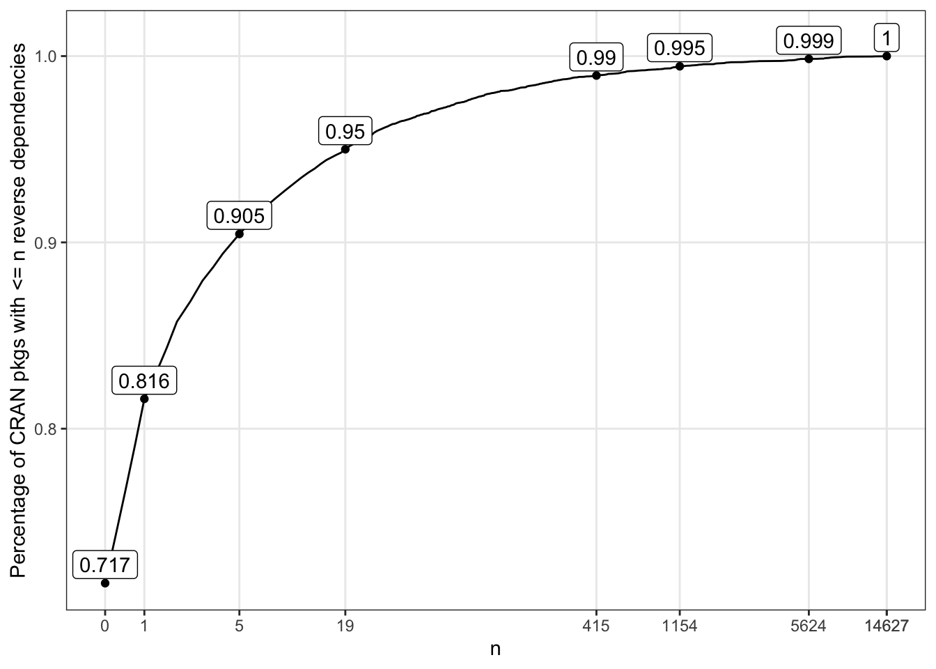

Whether you have guessed or not:

• 71.7% of CRAN packages don’t have any reverse dependency;
• fewer than 10% of the packages on CRAN have more than 5 reverse dependencies; and
• only 1% of the packages have more than 415 reverse dependencies

So while the majority of the R packages do not need reverse dependency checks, a small number of core packages need to test against hundreds or even thousands of reverse dependencies for every new release.

Alternatively, we can rank the packages by their number reverse dependencies (the package with the largest number of reverse dependencies is ranked first). The advantage of this is that there turns out to be a distribution that can capture the shape well: the Zipf–Mandelbrot distribution, the generalised zipf distribution, which is commonly used to model corpus frequency in linguistics:

Code

nodes_rank <- nodes %>%  
  mutate(rank = rank(-n_revdep, ties.method = "first")) %>% 
  filter(n_revdep > 0)

dt_pos <- nodes %>% filter(n_revdep > 0) %>% pull(n_revdep) %>% sort(decreasing = TRUE)
pred1 <- fitrad(dt_pos, "mand") %>% radpred()
fitted <- tibble(
  rank = pred1$rank,
  mand = pred1$abund, 
  count = dt_pos)

p2 <- nodes_rank %>% 
  ggplot(aes(x = rank, y = n_revdep)) + 
  geom_point_interactive(aes(tooltip = id)) + 
  geom_line(data = fitted, aes(x = rank, y = mand), color = "#314f40") + 
  ggrepel::geom_text_repel(
    data = nodes_rank %>% filter(n_revdep > 3100), 
    aes(label = id, color = category),
    min.segment.length = 0) + 
  scale_y_continuous(breaks = c(10, 50, 200, 500, 1000, 2500, 5000, 7500, 10000, 15000)) + 
  scale_x_continuous(breaks = c(0, 1, 10, 50, 100, 200, 500, 1000, 2000, 5000, 10000, 20000)) + 
  coord_trans(x = "log", y = "sqrt") + 
  scale_color_brewer(palette = "Set1") + 
  theme_bw() + 
  theme(panel.grid.minor = element_blank(), 
        legend.position = "bottom") + 
  ylab("number of reverse dependencies")
girafe(ggobj = p2, width_svg = 16, height_svg = 12)

Contender for the next isoband

We can also find packages with similar characteristics as isoband: those with a huge number of reverse dependencies (n > 3000) while not managed by base R or RStudio or listed as recommended on CRAN:

Package	# of reverse dependency
Rcpp	8401
fansi	6777
utf8	6777
digest	6418
colorspace	5041
RColorBrewer	5030
viridisLite	4895
farver	4875
labeling	4865
munsell	4864
stringi	4573
jsonlite	4326
yaml	3031
mime	3020

In a quick glance, these packages fall into three categories:

1. Color packages: colorspace, RColorBrewer, viridisLite, munsell
2. Super giants:

• Rcpp for interfacing to C++ for fast computation;
• jsonlite for parsing JSON; and
• stringi for string manipulation.

3. Hidden dependencies: These packages don’t have a huge number of direct dependencies themselves but is imported by a giant package:

• imported by ggplot2:
  • digest for hashing object in R, and
  • farver and labelling are imported by scales, which in turn is imported by ggplot2
• imported by tibble:
  • fansi for ANSI text formatting, and
  • utf8 for processing UTF encoding, imported by pillar, which is imported by tibble
• imported by shiny: mime for converting file name extension, and
• imported by knitr: yaml for YAML text conversion

The social network

Finally, the network diagram! I have tried to include all 17,354 nodes and 551,713 pairs of edges in a single diagram and I do not blame my computer for rejecting it with

vector memory exhausted (limit reached?). 

To avert this error, I plot a subset of the large number of packages with n ≤ 5 reverse dependencies. Specifically, for each n ≤ 5, I randomly select 40 packages with the given n. After playing around with layouts and other aesthetics, here is the result…

code

Code

wirdos <- c("brglm", "profileModel", "ExPosition", "prettyGraphs", "seasonal", "x13binary", "scalreg", "lars", "elasticnet")
more_than5 <- nodes %>% filter(n_revdep > 5) %>% filter(!id %in% wirdos)
set.seed(123)
less_than5 <- nodes %>% 
  filter(n_revdep <= 5) %>% 
  nest_by(n_revdep, .key = "nested") %>% 
  mutate(id = list(map(nested, ~sample(.x, size = 40))$id)) %>% 
  unnest(id) %>% 
  select(-nested) %>% 
  ungroup()

new_nodes <- bind_rows(more_than5, less_than5)
new_edges <- dep_lookup_tbl %>% filter(upstream %in% new_nodes$id & downstream %in% new_nodes$id) %>% select(-type)
new_nodes <- new_nodes %>% filter(id %in% c(new_edges$downstream, new_edges$upstream))
g <- tbl_graph(nodes = new_nodes, edges = new_edges, directed = TRUE)

ggraph(g, layout = "fr") + 
  geom_edge_link(alpha = 0.1) + 
  geom_node_label(data = ~ .x %>% filter(n_revdep >= 3200), aes(label =id), repel = TRUE) + 
  geom_node_point(aes(size = n_revdep), alpha = 0.5) + 
  theme_void() + 
  theme(legend.position = "none")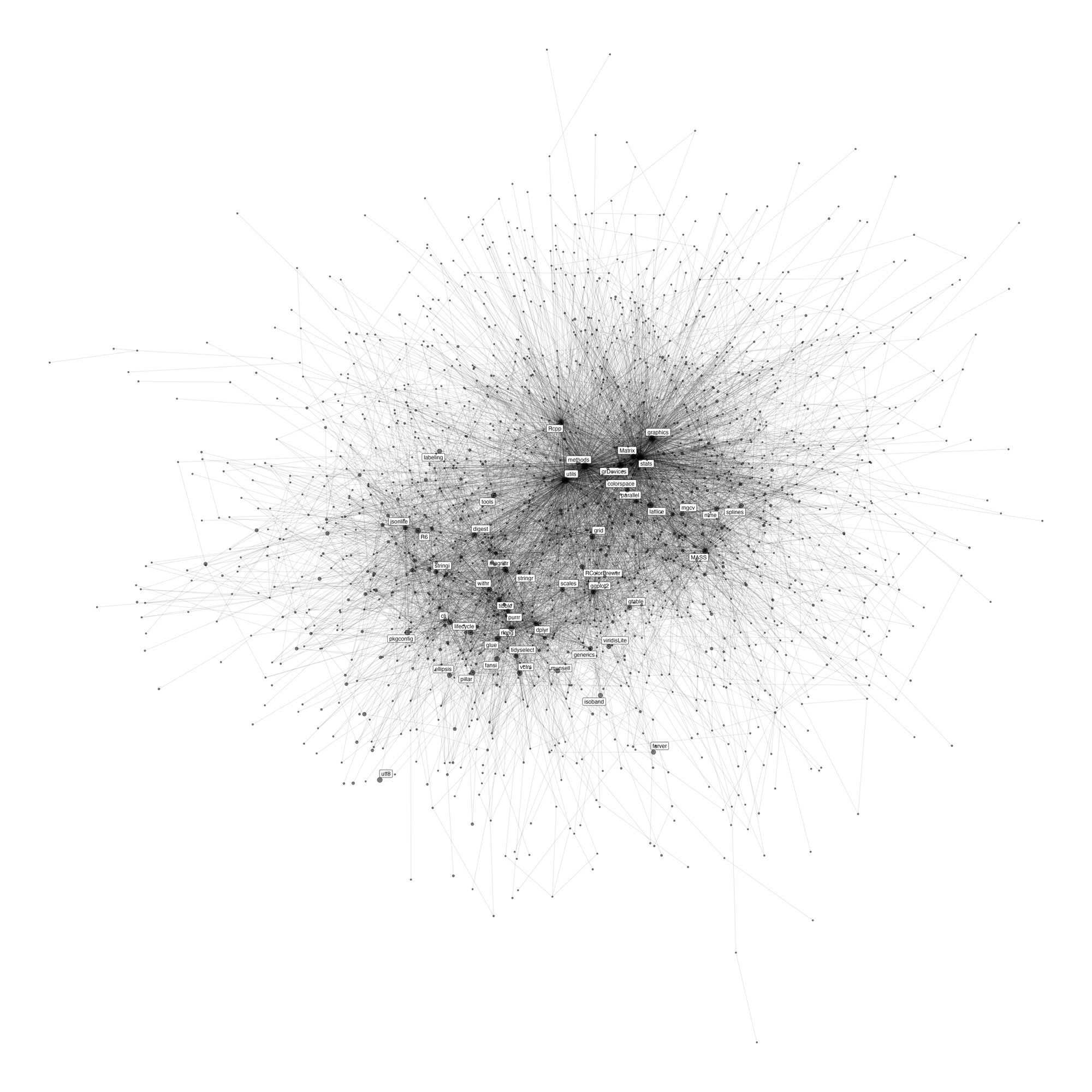

Footnotes

1. On 5th Oct, CRAN sent out a massive email to inform 4747 downstream package maintainers of the potential archive of package isoband on 2022-10-19.